Planning with Approximate Inference [3* P]

In this example we consider a 2-link planar arm. In this task you have to plan an optimal path from an initial joint-position to a given endeffector-position ¹² by Gibbs sampling.

The length of the links $l_1$ and $l_2$ is given by $0.5$ meters. We will restrict the first joint position of our arm model to be in the range of $[0; \pi/2]$ and the second to be in the range of $[-\pi / 2; \pi / 2]$ .

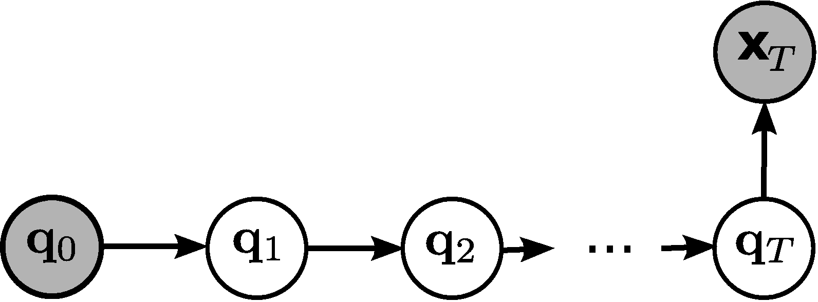
We will first discuss how to construct a Bayesian Network where we can sample from. We want to reach our target within $T=10$ time steps, i.e. we get a dynamic Bayesian Network with one node per time step (11 nodes), see Figure 10.

Figure 10: Dynamic Bayesian Network for task-space planning. The task-space is defined as cartesian coordinates of the endeffector position.

Each node $t$ represents the joint positions $\mathbf{q}_t$ at time $t$ . For simplicity, we will use a discrete representation of the joint positions. Therefore we use a uniform $11 \times 11$ grid to discretize the joint space. We will use a Gaussian motion prior in order to define the transition probabilities of $P(q_{t}^{(j)}\vert q_{t-1}^{(i)})$ from the $i$ th discrete joint position at time $t-1$ to the $j$ th joint position at time $t$ . Let $\mathbf{q}^(j)$ be the $j$ joint position vector (in radians), then $P(\mathbf{q}_{t}^{(j)}\vert\mathbf{q}_{t-1}^{(i)}) \propto \mathcal{N}(\mathbf{q}_{t}^{(j)}\vert \mathbf{q}_{t-1}^{(i)}, \mathbf{W})$ , where $W$ equals $\textrm{diag}([0.0125, 0.05])$ . The motion prior encodes our laziness, meaning that, if not necessary, we do not want to move away from $\mathbf{q}_{t-1}$ .

In order to plan a trajectory to a certain end-effector position we still need to define our kinematic task space mapping. We will also use a discrete representation for task space (Cartesian coordinates of the hand). Here, we use again a $11 \times 11$ uniform grid over the range $[0;1]$ for $x$ and $y$ . The probability of reaching the $j$ th discrete task space position when being in the $i$ th discrete joint space position is given by $P(x_t^{(j)}\vert q_t^{(i)}) \propto \mathcal{N}(x_t^{(j)}\vert \Phi(q_t^{(i)}), \mathbf{C})$ , where $\Phi$ is the non-linear mapping from the joint positions to the endeffector coordinates. The covariance matrix $\mathbf{C}$ is set to $\textrm{diag}([0.004, 0.004])$ .