Pseudo-Dynamic Planning with Obstacle Avoidance (Optional Task)

Try the approach also on a dynamic task.

Now we also want to add the velocities $\dot{\mathbf{q}}$ of the joints to our planning scenario. Therefore, we will also incorporate controls $\mathbf{u}$ of the robot in our model. The controls $\mathbf{u}$ directly represent the accelerations of the joints. The control-dependent state transitions are now given by

$$P(\mathbf{q}_t, \dot{\mathbf{q}}_t\vert\mathbf{q}_{t-1}, \dot{\ma... ...\mathbf{q}}_{t-1}; \dot{\mathbf{q}}_{t-1} + 0.1 \mathbf{u}_{t-1}], \mathbf{W}),$$

where $\mathbf{W}$ is set to $\textrm{diag}([10^{-5}, 10^{-5}, 10^{-3}, 10^{-3}])$ . Now, in difference to the previous tasks we incorporated controls to our model. For each dimension we will use $5$ discrete actions $u_{1,2} \in [-4, -2, 0, 2, 4]$ , resulting in a action space of $25$ actions. The actions are unknown, and hence, like every unknown hidden variable, they can be integrated out : $P(\mathbf{q}_t, \dot{\mathbf{q}}_t\vert\mathbf{q}_{t-1}, \dot{\mathbf{q}}_{t-1... ...t-1}, \dot{\mathbf{q}}_{t-1}, \mathbf{u}_{t-1}^{(i)}) P(\mathbf{u}_{t-1}^{(i)})$ . The term $P(\mathbf{u}_{t-1}^{(i)})$ denotes the action prior, similarly to the previous example we again use it to code our laziness, i.e. we prefer doing no action at all $P(\mathbf{u}_{t-1}^{(i)}) = \mathcal{N}(\mathbf{u}_{t-1}^{(i)}\vert, \mathbf{H})$ , where $\mathbf{H}$ is set to $16 \mathbf{I}$ .

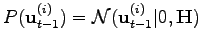
As we can see the controls are excluded from the inference process, however, they can be easily calculated from an estimated trajectory $[\mathbf{q}_{1:T}, \dot{\mathbf{q}}_{1:T}]$ . We will again use a discretization of the state space with a $11 \times 11 \times 11 \times 11$ uniform grid. Valid velocities are in the range of $[-1;1]$

• Create the state transition probabilities $P_{qq}$ for the dynamic case. Also create the task space mapping $P_{qx}$ and the collision mapping (both do not depend on the velocities). Use the same intial state and target end-effector position as before, but set the velocity to zero.
• Again use Gibbs sampling to sample from valid trajectories. Now use $50000$ Gibbs sampling steps and $1000$ steps between two independent samples. Again calculate the marginals and visualize the marginals of the positions $\mathbf{q}_t$ for each time step.
• In addition, plot the expected positions and velocities for each joint over time.