Approximate inference in Bayesian networks [3 P]

Apply Gibbs sampling to carry out approximate inference in Bayesian networks. You should estimate the (marginal) probability distribution of several variables in a Bayesian network, given the settings of a subset of the other variables (evidence). Implement the Gibbs algorithm in MATLAB based on the code provided Gibbs.zip¹¹ and test it on the three Bayesian networks shown below. Your code should run Gibbs sampling a specified number of iterations in order to estimate the required probability distributions. Since Gibbs sampling is a randomized, iterative algorithm, the actual number of iterations needed to estimate probabilities is an important issue, that will be explored as part of this assignment.

a)

Download the MATLAB code and modify the file gibbs.m to implement Gibbs sampling. The file loads one of six predefined Bayesian networks that are stored in the files alarm.mat, insurance.mat, leader-follower_05.mat, ... leader-follower_20.mat. Each of these data files contains the two variables var and p that specify the random variables and the factors of the joint probability distribution for each Bayesian network, respectively.

Figure: A Bayesian network establishing relations between events on the burglary-earthquake-alarm domain, together with complete specifications of all probability distributions.

b)

As a sanity check, to be sure that your code is working, start by running Gibbs sampling on the "earthquakes and burglar alarms" Bayesian network (Fig. 6) provided in the file alarm.mat.

1. Run Gibbs sampling 1000 times for 2000 steps starting each time from random intial values for the hidden variables (drawn from a uniform distribution) and verify that the conditional probability of burglary given that both John and Mary call is approximately 0.284. In order to estimate this conditional probability calculate the mean and the SEM (standard error of the mean) for the 1000 values of the binary random variable that is one if burglary = true and 0 otherwise (after 2000 steps).

2. Suppose now that you learn that there was an earthquake in the area. Run Gibbs sampling to estimate the probability of a burglary (given that John and Mary both called, and that there was an earthquake). Interpret the result.

Figure: A Bayesian network establishing relations between events on the automobile insurance domain.

c)

The Bayesian network illustrated in Fig. 7 attempts to estimate the risk posed by an individual seeking car insurance. In other words, the network attempts to relate variables like the age and driving history of the individual to the cost and likelihood of property damage or bodily injury.

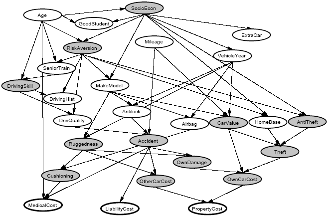
The network has 27 variables (usually the 12 shaded variables are considered hidden or unobservable, while the other 15 are observable) and over 1400 parameters. An insurance company would be interested in predicting the bottom three "cost" variables, given all or a subset of the other observable variables. The network has been provided in the file insurance.mat.

1. You should estimate the cost of property damage, i.e. the probabilities of the values of the variable PropertyCost, for an adolescent driving a car (Age = Adolescent) with about 50,000 miles (Mileage = FiftyThou) and no anti-lock brakes (Antilock = False).

   Run Gibbs sampling for a 1000 times for 1, 10, 100, and 1000 steps starting from random intial values for the hidden variables (drawn from a uniform distribution) and plot the dependence of the resulting probability distribution (obtained for the 1000 trials) on the number of steps. Because some of the factors of the joint probability distribution are 0 you have to make sure that the probability of the intial state of the random variables is larger than zero (if not choose another initial state).

   How long ist the burn-in time (number of steps) that is required to sample from the stationary probability distribution?

2. Try out at least one other query of your own invention and report the results. Comment on why your results did or did not make sense.

Figure: A Bayesian network establishing relations between events on the leader-follower domain.

d)

Explore the convergence properties of Gibbs sampling on a very simple family of Bayesian networks. Theoretically, Gibbs sampling will converge to the correct stationary probability distribution asymptotically, that is, as the number of iterations becomes very large. However, in practice, it is not always clear how many iterations actually suffice, as this example demonstrates.

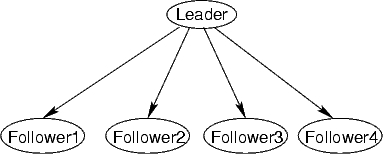
Each network in this family has a single "leader" variable, and some number of "follower" variables as shown in Fig. 8. The idea is that the leader selects a bit at random (0 or 1 with equal probability), and then all of the followers choose their own bits, each one copying the leader's bit with 90% probability, or choosing the opposite of the leader's bit with 10% probability. Leader-follower networks with $k$ followers have been provided in the files leader-follower-k.bn for $k = 5, 10, 15, 20$ .

What is the marginal probability distribution for the leader variable, in the absence of any evidence (i.e., none of the other variables have been set to specified values)?

1. What is the correct answer for the query given above? (This should be easy to answer.)

2. Run Gibbs sampling on a network with 5 followers using the given query. Run for at least 1000000 steps, printing the partial results every 1000 steps. Make a plot of the estimated probability (as estimated by Gibbs sampling) of the leader choosing the bit 0 as a function of the number of steps. In other words, the x-axis gives the number of steps, and the y-axis gives the probability of the leader bit being 0 as estimated after t steps of Gibbs sampling. Does Gibbs sampling seem to converge to the right answer? If so, roughly how long does it seem to take?

3. Now repeat the last question on networks with 10, 15 and 20 followers. Run for at least 1000000 steps, printing partial results at least every 1000 steps.

4. Can you explain what you observed? Why does Gibbs sampling have such a hard time with these networks? What do these experiments say about the difficulty of detecting convergence?

Submit your MATLAB code. Present your results clearly, structured and legible. Document them in such a way that anybody can reproduce them effortless.