Cart-Pole Controller Optimization [5 P]

Optimize the weights of a neural network that controls the horizontal forces applied to a cart in order to swing up a pole that is mounted on it into the upright position. Use an optimization algorithm of your choice (one of the four algorithms used in homework assignment 1). The state $\bf {x}$ of the dynamical system is defined as a four dimensional vector with the elements 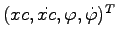$(xc,\dot{xc},\varphi,\dot{\varphi})^T$ , where $xc$ is the position of the cart and $\varphi$ is the pole angle.

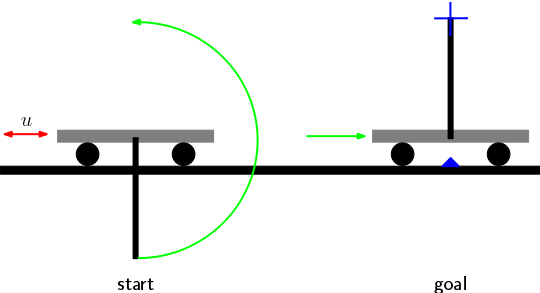
Figure: The cart-pole model.

a)

Download the MATLAB code for the cart-pole.² The dynamics of the cart-pole for one time step is computed in the function cp_dyn.m. The state $\bf {x}$ of the cart-pole can be visualized with the function cp_vis.m (you don't have to change or call these two functions).

b)

Modify the file learn_cp.m that contains also the parameters for the cart-pole in the structure model (masses, length of the pole etc.) to implement an optimization algorithm that minimizes the error computed with the function cost_function.m.

c)

Modify the file cost_function.m that simulates the cart for a duration of 10 seconds and assigns an error value to the dynamics of the cart. You have to i) complete the function cost_function.m to implement a neural network controller that generates the horizontal force $u$ that is applied to the cart at each time step, and ii) define an appropriate error function $e$ (that scores the cart-dynamics for each time step), which has to be minimized.

d)

Neural network controller: Write the code to initialize and simulate a neural network without using the neural network toolbox. The input to the network for each time step should consist of the following 5 values: 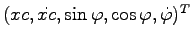$(xc,\dot{xc},\sin{\varphi},\cos{\varphi},\dot{\varphi})^T$ . Choose an appropriate number of hidden neurons for the single hidden layer. The scalar output of the neural network, i.e. the force, should be bounded with values between -10 and 10.

Hints: Don't forget to optimize the bias values of the neurons. Use a tansig output neuron to obtained bounded output values.

e)

Error function: Use the state variables to construct an error function $e$ that outputs a value at each time step that assure that the pole remains in the upright positions after the upswing. Set the error to $\infty$ if the cart leaves the interval $[-1,1]$ . The total error (or cost) assigned to the cart movement could e.g. be the sum of all $e$ for all time steps.

Hints: Take care of the fact that the values for $\varphi$ returned by the dynamical model in cp_dyn.m are not within the interval $[0, 2\pi]$ .

f)

Analyze the best solution found and state the reasons for all choices you made in the MATLAB code.

Present your results clearly, structured and legible. Document them in such a way that anybody can reproduce them effortless.